Web App for Deriving Stress Scenarios from the Yield Curve
The Web App uses the python-flask framework to perform a principal component analysis (PCA) of the yield curve, to visualize
the results and to derive adverse scenarios for stress testing. This document gives an overview of the used data, the regulatory context, the mathematical and technical setup,
a brief discussion, and an outlook for further development. The web app provides interactive access to the methodology
described in this document.
Deriving Stress Scenarios from the Yield Curve
In the valuation of assets and liabilities through future cashflows, yield curves play a central role.
A yield curve at a given time consists of multiple spot rates across maturities, and those rates tend to move
together over time. To create meaningful stress scenarios, it is essential to understand these common movements.
PCA provides that insight by reducing highly correlated, high‑dimensional data to a lower‑dimensional representation
with good approximation quality.
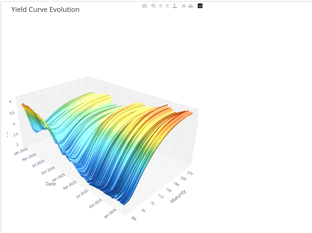
The Data
The yield curve over time can be plotted as a three‑dimensional surface. The x‑axis is time, the y‑axis is maturity,
and the z‑axis is the corresponding spot rate.
Regulatory Context
Many regulatory approaches state the importance of interest risk. The definition of interest rate risk in the
Solvency II Guideline says:
Article 105 – Calculation of the Basic Solvency Capital Requirement
The market risk module shall reflect the risk arising from the level or volatility of market prices of financial
instruments which have an impact upon the value of assets and liabilities of the undertaking. It shall properly
reflect the structural mismatch between assets and liabilities, in particular with respect to the duration thereof.
It shall be calculated, in accordance with point 5 of Annex IV, as a combination of the capital requirements for at
least the following submodules: the sensitivity of the values of assets, liabilities and financial instruments to
changes in the term structure of interest rates, or in the volatility of interest rates (interest rate risk).
The Solvency II standard formula demands one up and one down scenario of the yield curve; each leads to a revaluation
of the future cashflows from assets and liabilities. The International Association of Insurance Supervisors suggests
several stress scenarios which change the level, slope, and curvature of the yield curve. Modelling the fluctuations
in the yield curve is critical to quantify interest risk.
Technical Setup
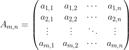
The yield curve can be described as a matrix of m historical observations, each with n dimensions. PCA computes
principal components from the covariance matrix and defines a new coordinate system based on those components.
The principal components form an orthonormal basis, so the transformation maps the centered yield curve into a
lower‑dimensional representation. The inverse mapping reconstructs an approximation of the original curve.
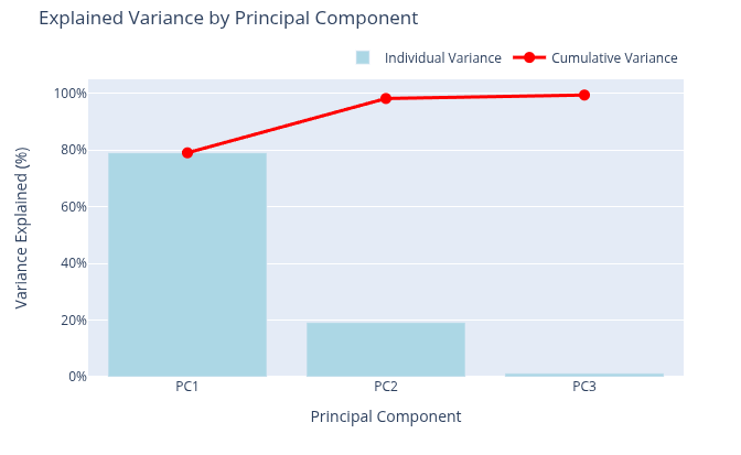
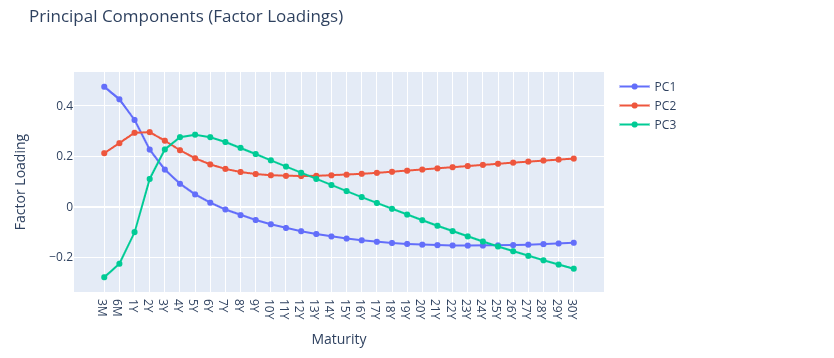
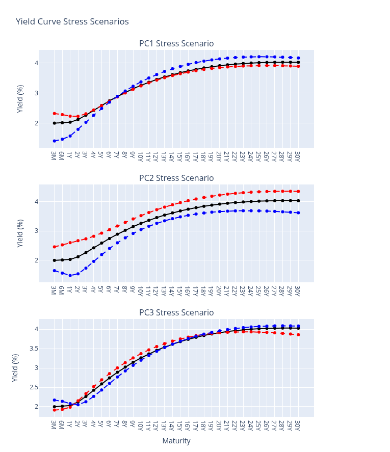
The scores are the coordinates in the new system. Most variance in the yield curve is explained by the level, so
the first three principal components typically capture the bulk of variation. PC1 is often associated with level,
PC2 with slope, and PC3 with curvature. Linear combinations of these three components provide a strong approximation
of the yield curve in terms of explained variance.
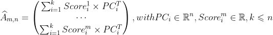
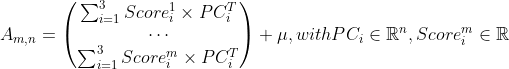
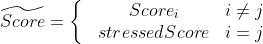
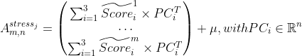
To construct a yield curve stress scenario from the scores, the PCA must be inverted. By construction the inverse
is the transpose of the component matrix. A stressed scenario can be created by replacing a component score with a
stressed value (for example a 99.5% quantile) and reconstructing the yield curve.
Discussion
Pro
- PCA derives effective models to represent high dimensional data with a low number of explaining variables.
- A simplified model of the yield curve using only a few uncorrelated random variables is achievable.
- PCA itself is a non‑parametric method, so it is not necessary to make assumptions about the distribution.
- Using the first components it is possible to create up/down stress scenarios for level, slope and curvature.
Contra
- PCA is still a correlation analysis, so a stationary time series is required.
- Explained variance is the only criterion for selecting principal components.
- Tail scenarios are limited to linear combinations of the chosen principal components.
- Results are not stable over time as supervisory measures and the yield curve shape can change.
- Using historical quantiles implicitly assumes future tail events will not exceed past tail events.
Technical Specifications
- Different target variables are possible: differences of spot rates, forward rates, or returns.
- Daily data was used, but monthly or hourly data is possible.
- A rolling timeframe of 24 months for calculating the 99.5% quantile of monthly changes was used.
- Shorter windows are more sensitive to recent outcomes; longer windows may include less relevant history.
- Tail events were not explicitly emphasized when choosing the number of PCs.
Further Development
- Calculate scenario severity with cashflow scenarios that depend on the shape of the yield curve.
- Include the occurrence of tail events explicitly.
- Compare results to other yield curve modelling techniques like Nelson‑Siegel.
- Extend the model to a PC‑GARCH model.
Literature
- Alexander (2002), Principal component models for generating large GARCH covariance matrix.
- EIOPA (2019), Consultation paper on the opinion on the 2020 review of Solvency II.
- European Commission (2015), Regulation 2015/35 and Directive 2009/138/EC (Solvency II).
- McNeil, Frey, Embrechts (2005), Quantitative Risk Management.
- Redfern, McLean, Moody's (2014), PCA for yield curve modelling.
- IAIS (2020), ICS Version 2.0 for the monitoring period.
- Schlütter (2020), Scenario‑based Measurement of Interest Rate Risks.